Retrieving specific information from a spreadsheet using a Combo Box and the VLOOKUP Function

You can click here to get an example starting spreadsheet.

Step 1: Create a Combo Box which uses values from another worksheet

Create a Combo box to select a name of a student whose details you want to bring up in the page. To do this

• click on View | ToolBars | Forms

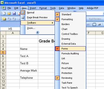
• Select a Combo box from the Forms toolbar and draw a Combo box.

• Right click on the Combo box and click on Format Control

• Make sure the Control tab is selected

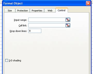
• In the Input Range Box enter the range of the table (on sheet 1) which contains all the names. However, note that you are entering the range in worksheet 2 but linking to the table on worksheet 1 hence the notation as below.

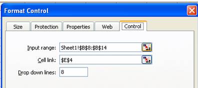
Sheet1!$B$8:$I$14

Sheet1! Identifies the link to the first worksheet, and $B$8:$I$14 is the range with absolute referencing. 

• Choose a cell link which will be used to provide a link between the worksheet 1 and information to be retrieved into the form created in worksheet 2:
  In cell link , enter $E$4 and click on OK

Once this is completed, you should be able to click on the Combo box and see the list of all the names of the students. Notice that when a name is selected, a cell link value appears in cell E4 which corresponds to the student number (the left most column of the table).

Step 2: Use VLOOKUP to retrieve specific values from another worksheet

Once a name has been selected from a drop down list, you want the grades for Test A, Test B and telephone details to automatically appear. To do this, you will use an Excel lookup function called VLOOKUP . This function is used to retrieve information stored in a worksheet elsewhere in the workbook.  

You can use this starting spreadsheet to practise this.  

When you use VLOOKUP, you need to enter 3 different cell ranges for it to work:

• lookup_value: The value to be found in a column which in this example is in cell E4
• table_array: The table of information in which the data is looked up.
• col_index_num: the numeric position of the column that is being searched.

Your formula would look like this (you will need to replace the writing in the brackets with the real information from your spreadsheet).

=VLOOKUP (lookup_value, table_array, col_index_num)

In the example spreadsheet do the following:

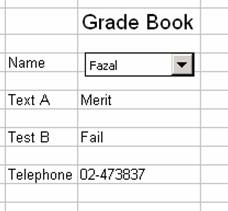
• Enter the VLOOKUP function in cell C6 as follows: =VLOOKUP(E4,Sheet1!A8:I14,6).
• Enter the VLOOKUP function in cell C8 as follows: =VLOOKUP(E4,Sheet1!A8:I14,9)
• Enter the VLOOKUP function in cell C10 as follows: =VLOOKUP(E4,Sheet1!A8:I14,3)

When you choose “Fazal” as the student whose details you want to see, the following information should appear:

Tip: you can make the cell link value in E4 invisible by making it the same colour as the background.